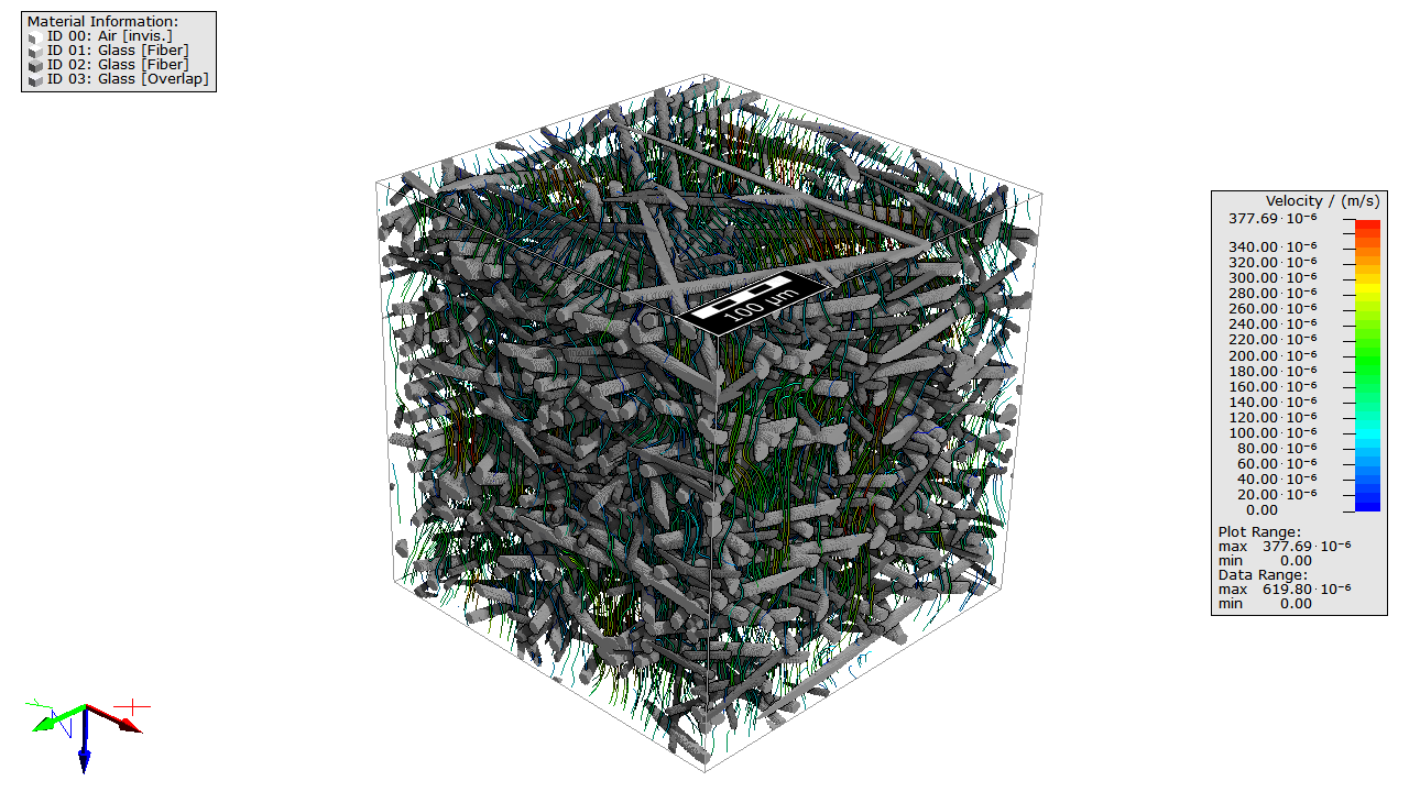
We will now use the results of the previous section to demonstrate how three-dimensional computational result fields (here: velocity and pressure) can be visualized. Here, we will visualize the flow field as streamlines.

For more detailed information about GeoDict's visualization options see the corresponding user guide.

1. Go to the Flow Visualization tab in the Result Viewer and click Load. In the opening dialog, click OK to load all data contained in the file
   
2. The volume field is now displayed in the visualization area of GeoDict. Switch to 3D rendering by clicking . Observe that the Volume Field and the Streamlines tabs have been enabled, above of the visualization area, in the View Controls panel. For now, navigate to the Camera tab.
   
3. For a nice visualization, first set the camera angle as desired. Enter -40 for Rotation HDG, -20 for Rotation ATT and 110 for Rotation BNK. These values define the camera angle precisely. When turning the structure with the mouse cursor, these values change accordingly. Thus, a position can be reached with the cursor and reproduced by entering the corresponding values for the rotation parameters.
   
4. Uncheck the Volume Field tab, as we only want to visualize the streamlines in this tutorial. Then, check the Streamlines tab.
   
5. Change to the Streamlines tab to modify the Line Thickness to 1.0.
   
6. We now want to save the current visualization as an image. To do that, select File → Save Image as… from the menu bar or click on the icon in the toolbar. In the opening dialog, check Preset and choose the desired resolution HD, 720p from the pull-down menu below.
   
7. Click OK and select a meaningful name. We chose Streamlines.png. The image is saved in the desired resolution to the project folder.