Results
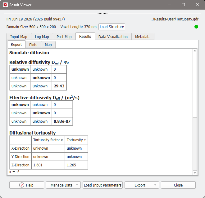
At the end of the computation, the Result Viewer of the Tortuosity.gdr result file appears automatically.
The Tortuosity Factor (1.6) and the Geometric Tortuosity (1.3) are found in the third table. As diffusion was only simulated in Z-direction, results for the other two directions are not available.
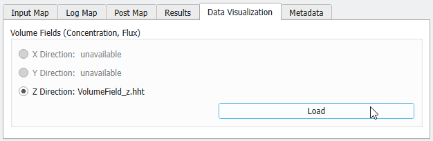
 Load Volume Field
To visualize the diffusion flux in 3D, select the Data Visualization tab and click Load.
In the Loading volume file dialog, leave all components checked to be loaded and click OK to close the dialog. If the visualization of the pore sizes from the previous chapter is still loaded the dialog additionally will have the option Keep existing Volume Fields. Leave this option unchecked, as we now only want to visualize diffusion.
|
Visualize Volume Field
In the GeoDict main GUI, uncheck the Structure tab above the visualization area.
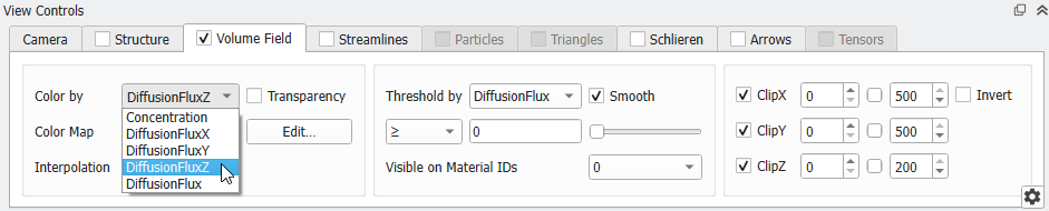
Select the Volume Field tab and for Color by choose DiffusionFluxZ from the pull-down menu.
Similar as done for the Porosimetry result from the previous unit, for Visible on Material IDs check ID 00 and deselect the two solid material IDs 01 and 02.
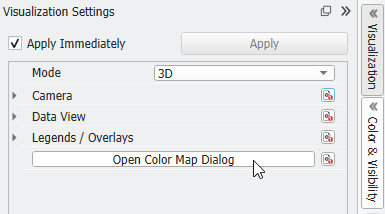
On the right, open the Visualization side bar and click on Open Color Map Dialog.
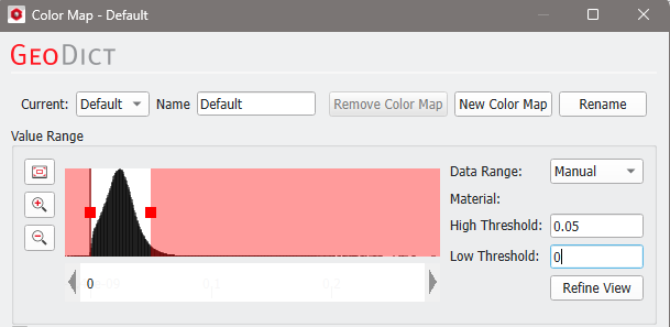
For Data Range select Manual. Now, it is possible to edit the lower and upper values for the data range. Set them to the following values: High Threshold to 0.05 and Low Threshold to 0.
If Apply Immediately is not checked, click Apply.
Close the dialog.
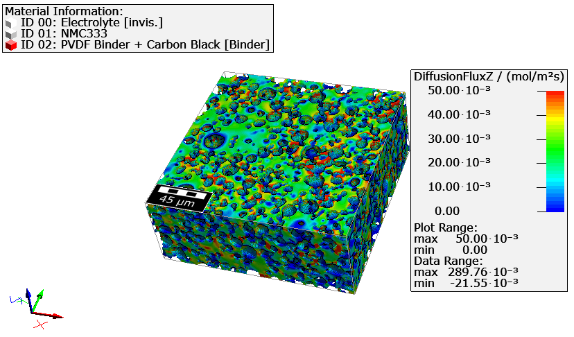
Now, the Diffusion Flux can be observed from all sides. Hot spots can easily be identified.
|
Visualization as Streamlines
Save Image
To save the visualization as an image from the menu bar select File → Save Image as.
In the opening dialog check Preset and choose the desired resolution from the pull-down menu below. We selected 1280 x 720, (HD, 720p). Click OK and select a meaningful name (we chose Tortuosity-Streamlines.png). The image is saved to the project folder.
|

 in the bottom right of the View Controls under the Streamlines tab.