To accelerate later operations, in the 3D Image Processing dialog, crop the image again by changing the values in the Crop NX and Crop NY boxes to 450 and 950 and click Apply. Thus, a smaller 500 x 500 x 200 data set will be imported, instead of the largest possible cutout obtained after the first cropping 1400 x 1400 x 200.
Of course, it is fine to work on the larger data if you can afford to spend more time and RAM in the following parts of this tutorial series. There, the cathode’s microstructure geometry and transport properties are analyzed. Based on the analysis a statistical digital twin is generated and validated.
To find out, if the chosen cut-out is representative for the properties to compute, proceed as outlined in step 3 Identifying a REV for geometric properties of the Digital Analysis of Battery Separator Structures tutorial, where REV stands for representative elementary volume.
Both cropping operations also could be done at once, using the values 774 and 1274 for Crop NX and Crop NY and 30 and 230 for Crop NZ.
The following step shows the difference resulting from the image filters and is optional. If you want to skip this visualization, after cropping continue with applying image filters.
Segment the gray scale image twice. First now, without the filters and again after applying the image filters.
To do so, back in the Image Processing dialog, switch to the Segmentation & Labeling tab on the left of the 3D Image Processing dialog and expand Global Thresholding. Change the Result File Name to ETH_NMC_Cathode-NoFilters.gdr.
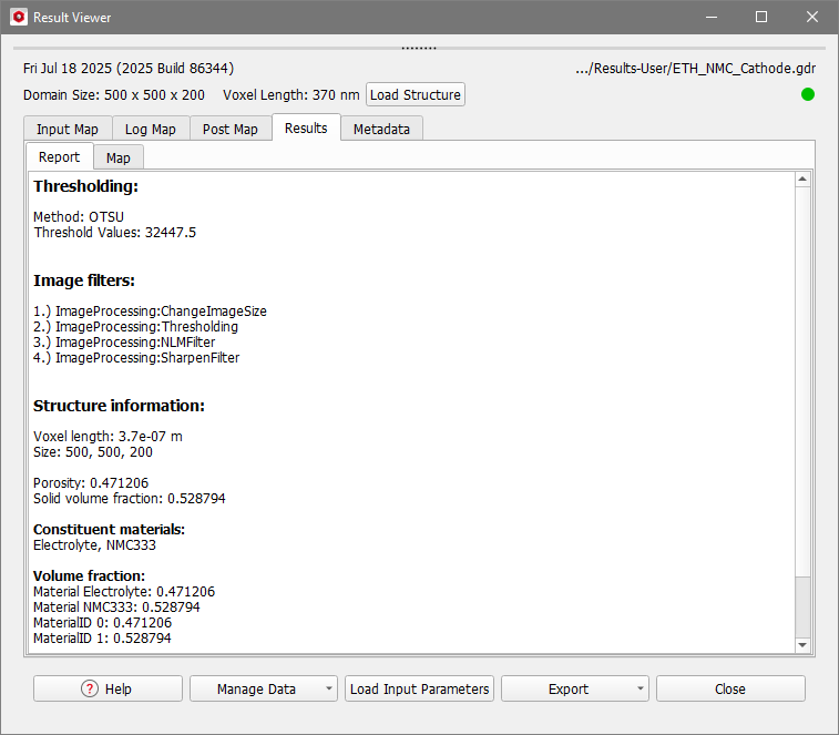
Now, click Create Segmentation at the bottom of the Global Thresholding section. The GeoDict result file saved by this import is the 2_ETH_NMC_Cathode-NoFilters_M2M.gdr included in the example data.
Under the Image Processing tab click the corresponding rotating triangle to display the Image Filters menu, and then the Non-Local Means Filter menu. Run the non-local means filter with the default settings by simply clicking Apply.
Then, change the Strength for the Sharpen Filter to 23 and click Apply.
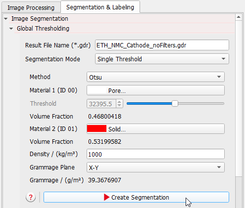
Move to the Segmentation & Labeling tab and unfold Image Segmentation and then Global Thresholding. There, change the Result File Name to ETH_NMC_Cathode.gdr.
Define the materials according to the scan. For this, click the button on the right of Material 1 (ID 00) to select Electrolyte as pore material. For Material 2 (ID 01) select NMC333 (Nickel-Manganese-Cobalt) as active material. Note, that Material 2 also contains binder and carbon black, but for now assigning it to NMC is good enough.
Continue by clicking Create Segmentation at the bottom of the Global Thresholding section. The GeoDict result file that is saved by this import is the 3_ETH_NMC_Cathode_M2M.gdr included in the example data.
In the 3D Image Processing dialog, click Discard Image in the bottom left to close the dialog and discard the gray value image from the GeoDict visualization area. In the opening dialog, click Yes.
Otherwise, the project folder Results-User now contains two result folders from importing the gray scale image. To compare the structures from the two folders we will subtract them from one another using the GeoDict module LayerGeo.
For this, the structure obtained from the import with image filters should still be displayed in the Visualization area of the GeoDict main GUI.
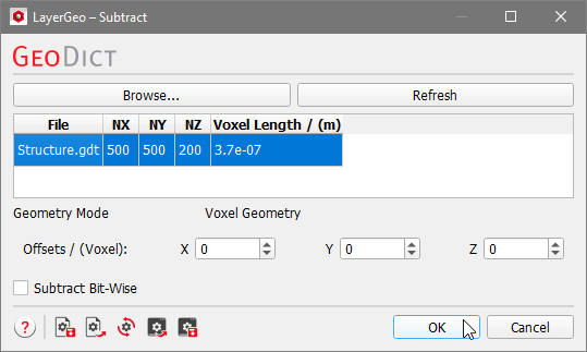
Select Model > LayerGeo from the menu bar. In the LayerGeo section, choose Subtract from the upper pull-down menu and click Edit....
In the opening dialog, click Browse… in the top left and select the folder ETH_NMC_Cathode-NoFilters. Click Select Folder.
Now in the LayerGeo – Subtract dialog a *.gdt file for the structure appears on the list. Select it.
Click OK to close the dialog, and then, click Run in the LayerGeo section of the main GeoDict GUI.
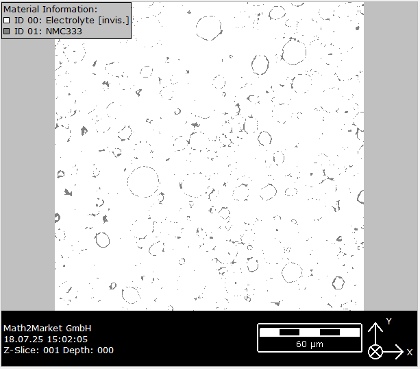
The resulting structure displays the difference between the filtered 3D image and the non-filtered. This way the effect of the filtering can easily be visualized and quantified. To visualize the result in 2D select View > 2D Cross Section (SEM) from the menu bar. How to display the structure with the colors and the visualization settings shown in this tutorial is described below.
To save this result select File > Save Structure as and enter Subtract.gdt as a name.
To go on working with the cathode structure, load the structure again by selecting File > Open Structure (*.gdt, *.gad) from the menu bar. Open the folder ETH_NMC_Cathode from the project folder. Select the Structure.gdt file and click Open.
Now, the structure is ready to be analyzed in GeoDict. For some properties it is necessary to additionally segment the binder from the NMC particles. For this, in the second part of this tutorial series a neural network is used to identify the binder phase.
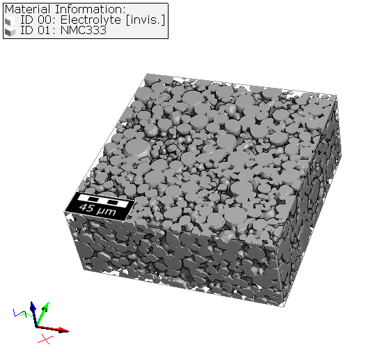
Now, the visualization settings can be changed to display the structure with the colors and the visualization settings shown in this tutorial.
Visualize the structure in 3D by clicking the icon in the toolbar or select View > 3D Rendering from the menu bar.
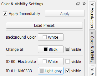
In the side bar of the GeoDict GUI, select Color & Visibility.
Change the color for ID 01: NMC333 from Red to Light gray. Click to exit the Color & Visibility Settings dialog.
Select the Camera tab, in the View Controls, above the Visualization area and check Show Outlines, Show Halo and Shadows to improve contrast. For the camera position used in this tutorial enter
-20 for Rotation HDG,
-8 for RotationATT and
-46 for RotationBNK.
0 for the translation and other rotation parameters.
Select the Structure tab, in the View Controls, above the Visualization area and from the pull-down menu for Structure Renderer select Smooth.
If you imported the complete data set (1400 x 1400 x 200) instead of the cropped (500 x 500 x 200) data set, the displayed structure looks as follows:
Figure: Visualization of the structure model created from the imported original data set of 1400 x 1400 x 200 voxels. The red rectangle marks the cropped 500 x 500 x 200 voxels, visualized on the right.

 Compare the two segmented structures
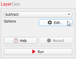
 to exit the Color & Visibility Settings dialog.