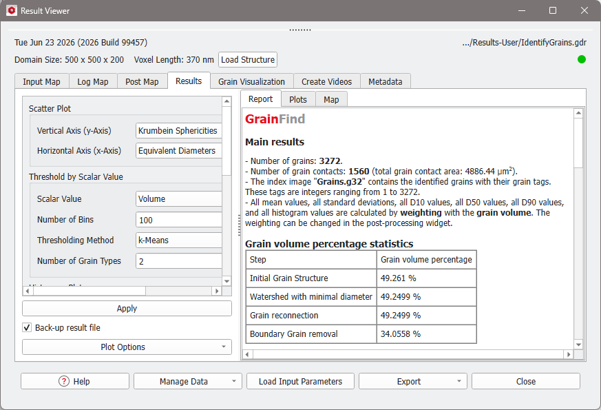
Select the Results - Plots subtab. By right-clicking on the scatter plot, and then selecting Save Image, you can create the image that is shown in the 6-1_grainShapePlot_M2M.png file in the example folder Results-M2M. In the opening dialog choose a meaningful Filename and a resolution. Find the resolution we used in the screenshot below. Then, click OK. The corresponding image is then found in the Results-User folder.
In the Result Viewer, change to the Grain Visualization tab. Visualize the identified Grains as Index Image by clicking Load *.g32. In the opening dialog click OK and leave the structure visible by clicking No in the message dialog.
Clip the structure to make the index image visible. For this, move to the Structure tab above the visualization area and set the Clip values as follows:
Clip X: 0-500
Clip Y: 320-500
Clip Z: 0-190.
Disable Invert
Each grain has its own number in the index image. The grains touching the boundary in the original structure cannot be found in the index image, since Remove Grain Fragments at Domain Boundary was checked in the Identify Grains Options dialog. The grain index number can be seen in a tool tip when hovering the mouse over the grain's voxels.
Through the *.g32 index image the material of single grains can be changed. For this, in the toolbar click the Select Voxels icon.
Then, on the right the Voxel Selection tab of the side bar opens.
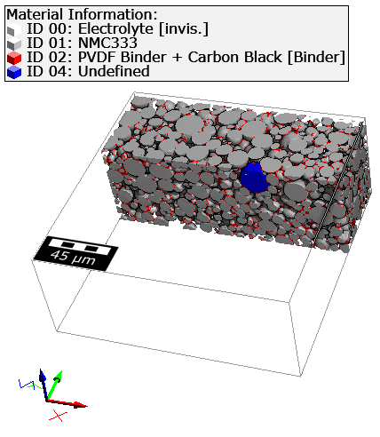
In the visualization area, select one voxel for each grain to change. Here, the same grain is selected as shown in the figure above. For Component Mode select Reassign Material of Objects (*.g32) and select a New Material ID, e.g., 04.
After clicking Run, the grain with the selected object ID, here 2822, has material ID 04.
To see the result, the Volume Field is automatically deselected in the View Controls.
To visualize how well the grains are fitted load Comparison of Segmented Grains and their Fits by clicking Load *.gdt in the Result Viewer.
Switch to the 2D view by clicking the 2D icon in the toolbar.
In the Camera tab of the View Controls, above of the visualization area, select the Direction for the view (here X) and scroll through the slices with the slider.
If the colors were set as described here, the fitted grains are visualized in red and the original grain material in light gray. The overlap is dark gray. Observe that most of the material is dark gray, which shows that the grains were fitted very well. This can also be verified in the Statistics bar in the project status section on the left.
For the current 2D slice in the 2D section (here for the X-slice 100) the statistics are shown in the figure below (on the left). After switching to the 3D view you can view the statistics for the complete structure. They are shown on the right in the figure below. For the complete structure, the not fitted original material is only 1.32 % of the volume (500x500x200 voxel) and only 1.31 % of the complete volume is wrongly fitted material, while the rightly fitted material is 32.73 % of the complete volume.
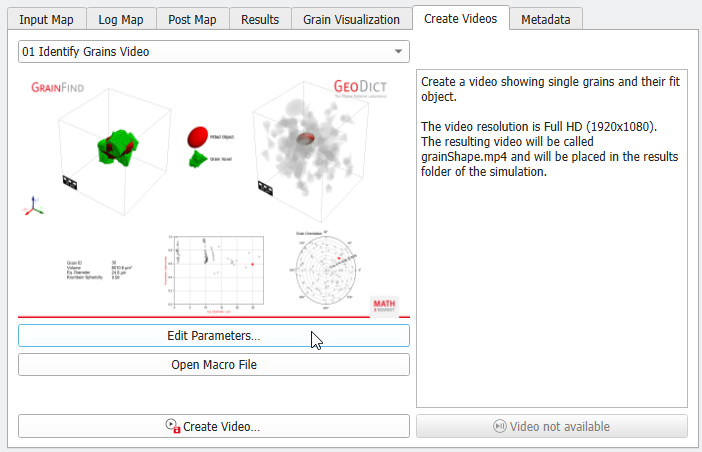
In the Result Viewer, switch to the Create Videos tab.
If you wish the video to contain the analysis of more than three grains (default), click Edit Parameters.
In the opening dialog, e.g., change the Number of Grains to 5 and the Approx. Video Duration to 10. This way, you obtain the same video found in the 6-2_grainShape_M2M.mp4 file in the example folder Results-M2M, which shows another grain every two seconds.
Click OK to close the dialog. To generate the video with the selected parameters, click Create Video.
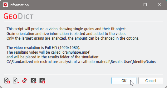
In the opening dialog giving information about the video creation and the movie file destination, click OK.
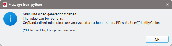
After about 15 minutes, a dialog appears, informing, that the video is finished and where to find it. Click OK to close the dialog.
The video can also be played back from the Result Viewer by clicking Play in the Create Videos tab.
Learn how the video is created through the script by clicking Open Macro File. To learn more about editing GeoDict macro files, refer to the GeoPy Scripting User Guide.
Now, the last animated grain is displayed in the GeoDict visualization area. To proceed with the cathode structure again, click Load Structure in the Result Viewer.
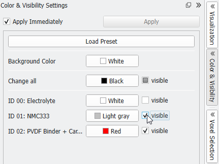
To visualize ID01 again, unfold the Color & Visibility Settings side bar and check visible for NMC333 again.
 Visualize Individual Grains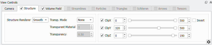

 in the toolbar.