CFD Simulation
created by Tina Jäger, technically reviewed by Dr. Sven Linden
What are CFD Simulations?
Fluid flow is everywhere - from the air flowing around an airplane to the water moving through a pipe. To understand and predict such flows, scientists and engineers use Computational Fluid Dynamics (CFD), also known as numerical fluid mechanics.

CFD is a numerical method used to simulate and analyze how gases and liquids move and interact with their surroundings. It allows the prediction of:
- Fluid flow – for example, air around an aircraft or water through a filtration membrane.
- Heat transfer – how temperature is distributed within a flow, such as the cooling of a hot engine by air.
- Chemical reactions – for instance, adsorption and desorption processes of pollutants in air or water.
The results of a CFD simulation typically include the distribution of pressure and velocity. Depending on the system, it can also include additional quantities such as temperature or concentration of chemical species.

CFD is an essential tool in design and research, helping engineers optimize systems and gain a deeper understanding of material behavior.
Why use CFD?
CFD simulations are used to predict how systems behave before they are physically built. This approach saves both time and cost compared to experimental testing.
For example, when developing an aircraft, engineers use CFD to understand how air flows around the structure and how design changes affect performance. Without simulation, such insights would require extensive and expensive wind tunnel experiments.
In material development, CFD also plays a crucial role. Consider wire meshes used in filtration or flow control: before manufacturing, engineers can create a digital model of the mesh and run a flow simulation. This allows them to evaluate performance parameters, such as pressure drop or flow patterns, under various design conditions.
By performing parameter studies, CFD enables the identification of optimal geometries and operating conditions without the need for multiple costly prototypes. As a result, CFD is an invaluable tool for both design optimization and process understanding.
How does CFD simulation work?
The fundamental basis of Computational Fluid Dynamics (CFD) lies in the mathematical description of fluid motion through the Navier–Stokes equations. These equations, developed in the 19th century by Claude-Louis Navier and George Gabriel Stokes, describe how velocity, pressure, temperature, and density of a fluid change in space and time.
Navier–Stokes Equations
In total, the full Navier–Stokes equations consist of four equations representing the conservation of mass, momentum, and energy and a closed by the equation of state. For most engineering applications involving liquids or slow gas flows, the incompressible form of these equations is sufficient.
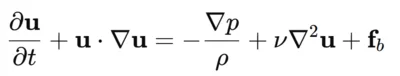
- The continuity equation (or mass conservation) ensures that mass is neither created nor lost within the flow domain.

These equations form a system of nonlinear partial differential equations. Because of their complexity, no general analytical solution exists, meaning they must be solved numerically.
Discretization of the Flow Domain
To make the problem solvable on a computer, the flow domain is divided into a finite number of small cells, called control volumes. The governing equations are then expressed in discrete form for each cell, and the solution in one cell depends on its neighboring cells.
Different CFD software tools use different spatial discretization methods, such as voxels, tetrahedra, or triangular elements for two-dimensional cases. Common numerical methods include:
- Finite Volume Method (FVM): The most widely used approach in CFD, based on the integral form of the conservation equations and known for its conservative properties.
- Finite Difference Method (FDM): Uses the differential form of the equations and approximates derivatives by differences between neighboring grid points.
- Finite Element Method (FEM): Less common in CFD but frequently used in solid mechanics (e.g., Abaqus); it can still be applied in flow simulations for specific applications.
The choice of method depends on the type of problem, the geometry, and the desired accuracy.
Iterative Solution Methods
After discretization, CFD solvers must iteratively solve large systems of linear or nonlinear equations. Various numerical algorithms are used for this purpose, such as Jacobi, Gauss–Seidel, or Multigrid methods for linear systems, and Newton-Krylov based methods for nonlinear problems.
The process continues until convergence is reached, meaning that:
- The solution variables (e.g., pressure, velocity) no longer change significantly between iterations.
- The residuals, i.e., the differences between the two sides of the equations, fall below a defined threshold.
- The quantities of interest, such as pressure drop, drag, or temperature, remain stable with further iterations.

The CFD simulation process
Although CFD simulations are used for a wide variety of problems, they all follow the same basic steps - from defining the problem to interpreting the results.
Step 1: Problem Identification
Every successful CFD simulation begins with a clear project definition. It is essential to know what result is expected - for example, the pressure drop, mass flow rate, or mean velocity.
The next step is to define the flow domain. You need to extract the region of interest rather than trying to simulate the entire system, since simulating everything is computationally expensive.
The scale of the simulation also needs should be chosen. Depending on the objective, this could range from:
- a single fiber (e.g., analyzing the flow around one filament),
- a cut-out from a fibrous media,
- a single pleat of a filter,
- an entire filter or battery,
- up to room scale simulations.

For heterogeneous materials such as nonwovens, a representative volume element (REV) can be identified - large enough to capture essential features, but small enough to be computationally feasible.
Simplifications are often applied, such as using symmetry conditions or assuming Stokes flow instead of the full Navier–Stokes equations when inertial effects are negligible. In many cases, the time-derivative can be dropped, leading to the solution of a steady state.
Step 2: Pre-Processing
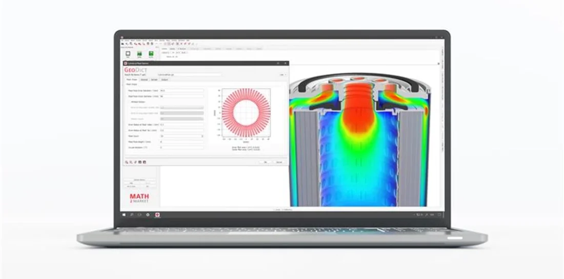
Pre-processing prepares the model for numerical simulation. In GeoDict, this involves defining the geometry together with its materials.
- Adjust the resolution to ensure that the imported geometry has sufficient resolution so that all geometric features can be accurately represented by voxels.
- Each component of the model should be defined as a separate object, allowing a specific material to be assigned later.

- The image data must be segmented to clearly distinguish between solid and pore regions. This segmentation step is essential for correctly identifying the flow domain. It ensures that the software recognizes which areas are permeable to fluid flow and which represent the solid matrix.
- Depending on the specific simulation, it may be important to segment the gray values into different material phases. This allows to setup up different material properties for each material phase

- When no physical sample or scan is available, stochastic modeling tools can be used to create digital twins. These models can reproduce statistically representative structures, such as nonwovens, foams, or fibrous filters, and serve as the computational domain for CFD analysis.
- GeoDict provides a suite of modules for Digital Material Design, including specialized structure generators like FiberGeo for fiber media, GrainGeo for granular and sintered materials, FoamGeo for open- and closed-cell foams, and WeaveGeo for woven fabrics. Additional structure-related modules like GridGeo for lattices and regular structures and PaperGeo for cellulose fibers exist, alongside tools such as GadGeo, LayerGeo, and ProcessGeo that aid in manual construction, modification, and combination of 3D microstructure models.
Step 3: Solving
Once the model setup and pre-processing are complete, the next step is to configure and run the solver. This stage involves defining the material properties, physical models, boundary conditions, and numerical parameters that govern the simulation process in GeoDict.

The first step is to specify the materials involved in the simulation. Depending on the problem, these can include:
- Fluids, such as air, water, or oil, with defined viscosity and density.
- Solids, which define the boundaries of the flow domain or interact with the fluid.
- Mixtures, representing porous media or composite materials.
GeoDict provides an extensive material database containing material constituents and their physical properties, which simplifies this step and ensures consistency across simulations.
The user must then select the relevant physical phenomena to be modeled. Depending on the application, this could include:
- Turbulence models for high Reynolds number flows.
- Combustion or multiphase flow models when chemical reactions or multiple interacting fluids are involved.
- The choice of the governing equations - for instance, solving the full Navier–Stokes equations or a simplified Stokes flow if inertial effects can be neglected.
The boundary conditions are important to model the desired experiment, and they define the behavior at the domain boundary or at material interfaces where assumptions must be made.
- Define domain boundary conditions (e.g., inlet, outlet, symmetry, or periodicity) together with prescribed values (such as velocity or pressure).
- Define interface boundary conditions (e.g., no-slip or slip) to model the behavior at the interface between materials.
During computation, the solver runs iteratively, updating the solution at each step. To ensure both accuracy and computational efficiency, appropriate termination criteria must be defined. These can include:
- A maximum number of iterations,
- A target residual level, representing how closely the equations are satisfied, or
- A tolerance threshold for key quantities such as pressure or velocity.
- GeoDict allows users to monitor the simulation in real time, observing how variables such as pressure or velocity evolve and ensuring that convergence is progressing correctly.
Step 4: Post processing
After the numerical solution has converged, the final step is post-processing - the examination, visualization, and interpretation of the simulation results. This stage transforms raw data into meaningful physical insights.
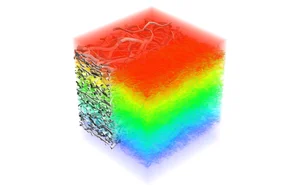

Visualization is a key component of CFD analysis, as it enables an intuitive understanding of complex flow behavior. In GeoDict, a wide range of visualization options are available to explore the results in detail:
- Identify the overall flow pattern and assess whether major flow features are correctly captured.
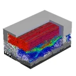
- Visualize the pressure and velocity fields to locate regions of high or low flow resistance.
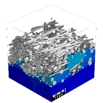
- Examine the simulation layer by layer to analyze variations within the material or geometry.
- Compute and visualize derived quantities such as the permeability tensor and viscous resistivity, which characterize material properties and flow performance.
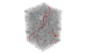
- Identify dominant flow paths that indicate preferred transport directions through porous structures.
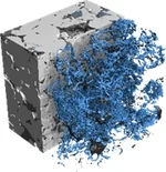
- Make vortices and recirculation zones visible to understand local flow instabilities or areas of energy loss.
Beyond visualization, quantitative evaluation is essential. Parameters such as pressure drop, mass flow rate, or local velocity distribution can be extracted and compared with experimental data or design specifications. These analyses form the basis for optimizing material structure, geometry, or operating conditions in subsequent development steps.
Through careful post-processing, CFD simulations evolve from numerical data into actionable engineering knowledge, allowing researchers and engineers to validate designs, refine materials, and gain deeper insight into complex flow phenomena.
Applications in industry
CFD simulations are applied across a wide range of industries and research areas to optimize designs, improve performance, and understand material behavior in detail. The following examples illustrate typical application fields of CFD.


Aerospace Engineering
Analysis of airflow around aircraft to determine lift and aerodynamic drag.
Automotive Industry
Simulation of engine cooling and vehicle aerodynamics
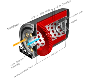
Filtration Technology
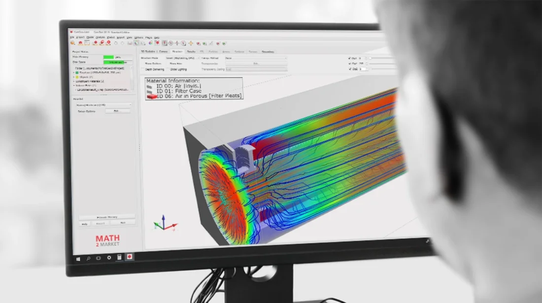
Prediction of filtration efficiency, capacity, and lifetime for various filter media such as air and gas filters, filter pleats
Oil & Gas / Digital Rock Physics
Simulation of two-phase fluid flow properties, including relative permeability, relative conductivity, and capillary pressure curves
Fuel Cells (PEMFC / SOFC)
Modeling of saturation-dependent transport properties and water management in Gas Diffusion Layers (GDLs), focusing on relative diffusivity and relative conductivity to optimize fuel cell efficiency and durability.
Environmental Engineering
Simulation of adsorption-based processes for the removal of pollutants from air or water
Technical Textiles and Membranes
Prediction of watertightness and liquid entry pressure of membranes and nonwovens
Advantages of CFD Simulation
CFD simulation offers several key advantages compared to traditional experimental methods:
- Lower Costs
Conducting laboratory or wind tunnel experiments is often expensive and time intensive. CFD simulations can be performed faster and at significantly lower cost, especially in early design phases. - Fewer Physical Tests
Because flow and transport processes can be predicted virtually, CFD reduces the number of physical experiments needed. Real tests are mainly used for validation, not exploration. - High Flexibility
CFD simulations make it possible to test new and unconventional designs that would be difficult or impractical to study experimentally. This accelerates innovation and supports concept evaluation. - Detailed Results
The method provides local and time-resolved data on velocity, pressure, temperature, or concentration - information that is often hard to measure experimentally. - Improved Understanding and Optimization
The visualization of flow and transport phenomena helps engineers understand why a design performs as it does. This insight simplifies corrections, performance assessment, and optimization.
In combination, these aspects make CFD a powerful and efficient complement to experimental research, enabling faster, deeper, and more cost-effective material and process development.


CFD Software GeoDict
GeoDict is an advanced software platform developed by Math2Market GmbH for the digital modeling, simulation, and optimization of materials and processes. It provides a complete environment for 3D image-based modeling and multi-physics simulation - from microstructure generation to property prediction.
A key advantage of GeoDict’s CFD functionality is that it operates directly on voxel data, meaning no meshing (grid generation) is required. This voxel-based approach significantly reduces pre-processing effort and allows a direct link between image data (e.g., from CT scans) and simulation. Combined with a user-friendly graphical interface, it makes CFD simulations intuitive and efficient.
GeoDict’s flow simulations are primarily focused on the microscale, where the flow through porous materials or small structures is analyzed. Typical applications include filter media, nonwovens, membranes, or rock samples. It is not intended for large-scale aerodynamic simulations of entire aircraft or vehicles.
Through a combination of voxel-based modeling, specialized solvers, and efficient algorithms, GeoDict can simulate large structures on standard computing hardware.
Are you interested in exploring CFD simulations and digital material development with GeoDict? Math2Market offers a free trial license that allows you to test the software’s capabilities and experience its workflow first-hand.
With the trial version, you can:
- Import and visualize 3D structures,
- Perform CFD simulations,
- Explore modules such as FlowDict or FilterDict, and
- Evaluate how GeoDict supports your research or product development tasks.
To request your trial license or learn more about GeoDict’s features, visit our page